How to turn your dog’s nap time into a regularized linear model

Looking at this nap duration model, Beta 0 is the intercept, the value the target takes when all features are equal to zero.

The remaining betas are the unknown coefficients which, along with the intercept, are the missing pieces of the model. You can observe the outcome of the combination of the different features, but you don’t know all the details about how each feature impacts the target.

Once you determine the value for each coefficient you know the direction, either positive or negative, and the magnitude of the impact each feature has in target.

With a linear model, you’re assuming all features are independent of each other so, for instance, the fact that you got a delivery doesn’t have any impact on how many treats your dog gets in a day.

Additionally, you think there’s a linear relationship between the features and the target.

So, on the days you get to play more with your dog they’ll get more tired and will want to nap for longer. Or, on days when there are no squirrels outside your dog won’t need to nap as much, because they didn’t spend as much energy staying alert and keeping an eye on the squirrels’ every move.

For how long will your dog nap tomorrow?

With the general idea of the model in your mind, you collected data for a few days. Now you have real observations of the features and the target of your model.

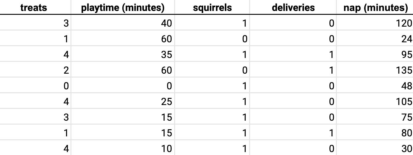
But there are still a few critical pieces missing, the coefficient values and the intercept.

One of the most popular methods to find the coefficients of a linear model is Ordinary Least Squares.

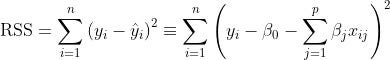
The premise of Ordinary Least Squares (OLS) is that you’ll pick the coefficients that minimize the residual sum of squares, i.e., the total squared difference between your predictions and the observed data[1].

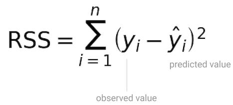
With the residual sum of squares, not all residuals are treated equally. You want to make an example of the times when the model generated predictions too far off from the observed values.

It’s not so much about the prediction being too far off above or below the observed value, but the magnitude of the error. You square the residuals and penalize the predictions that are too far off while making sure you’re only dealing with positive values.

This way when RSS is zero it really means prediction and observed values are equal, and it’s not just the bi-product of arithmetic.

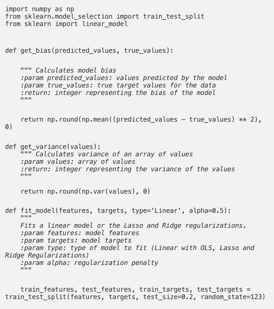
In python, you can use ScikitLearn to fit a linear model to the data using Ordinary Least Squares.

Since you want to test the model with data it was not trained on, you want to hold out a percentage of your original dataset, into a test set. In this case, the test dataset sets aside 20% of the original dataset at random.

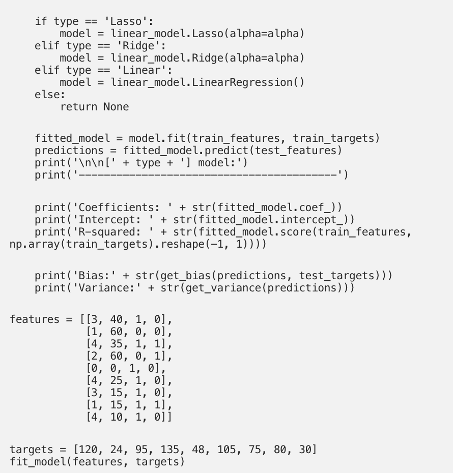
After fitting a linear model to the training set, you can check its characteristics.

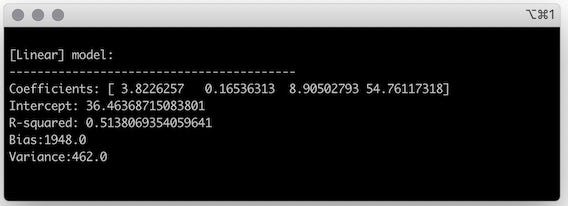
The coefficients and the intercept are the last pieces you needed to define your model and make predictions. The coefficients in the output array follow the order of the features in the dataset, so your model can be written as:

It’s also useful to compute a few metrics to evaluate the quality of the model.

R-squared, also called the coefficient of determination, gives a sense of how good the model is at describing the patterns in the training data, and has values ranging from 0 to 1. It shows how much of the variability in the target is explained by the features[1].

For instance, if you’re fitting a linear model to the data but there’s no linear relationship between target and features, R-squared is going to be very close to zero.

Bias and variance are metrics that help balance the two sources of error a model can have:

• Bias relates to the training error, i.e., the error from predictions on the training set.
• Variance relates to the generalization error, the error from predictions on the test set.

This linear model has a relatively high variance. Let’s use regularization to reduce the variance while trying to keep bias a low as possible.

Model regularization

Regularization is a set of techniques that improve a linear model in terms of:

• Prediction accuracy, by reducing the variance of the model’s predictions.
• Interpretability, by shrinking or reducing to zero the coefficients that are not as relevant to the model[2].

With Ordinary Least Squares you want to minimize the Residual Sum of Squares (RSS).

But, in a regularized version of Ordinary Least Squares, you want to shrink some of its coefficients to reduce overall model variance. You do that by applying a penalty to the Residual Sum of Squares[1].

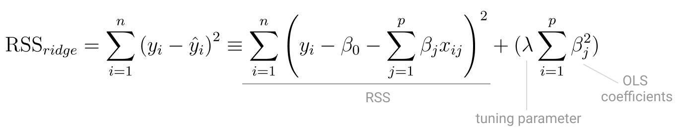
In the regularized version of OLS, you’re trying to find the coefficients that minimize:

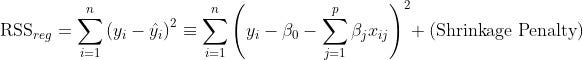
The shrinkage penalty is the product of a tuning parameter and regression coefficients, so it will get smaller as the regression coefficient portion of the penalty gets smaller. The tuning parameter controls the impact of the shrinkage penalty in the residual sum of squares.

The shrinkage penalty is never applied to Beta 0, the intercept, because you only want to control the effect of the coefficients on the features, and the intercept doesn’t have a feature associated with it. If all features have coefficient zero, the target will be equal to the value of the intercept.

There are two different regularization techniques that can be applied to OLS:

• Ridge Regression,
• Ridge Regression

  Ridge Regression minimizes the sum of the square of the coefficients.

  It’s also called L2 norm because, as the tuning parameter lambda increases the norm of the vector of least squares coefficients will always decrease.

  

  Even though it shrinks each model coefficient in the same proportion, Ridge Regression will never actually shrink them to zero.

  The very aspect that makes this regularization more stable, is also one of its disadvantages. You end up reducing the model variance, but the model maintains its original level of complexity, since none of the coefficients were reduced to zero.

  You can fit a model with Ridge Regression by running the following code.

  fit_model(features, targets, type='Ridge')

  Here lambda, i.e., alpha in the scikit learn method, was arbitrarily set to 0.5, but in the next section you’ll go through the process of tuning this parameter.

  Based on the output of the ridge regression, your dog’s nap duration can be modeled as:

  

  Looking at other characteristics of the model, like R-squared, bias , and variance, you can see that all were reduced compared to the output of OLS.

  

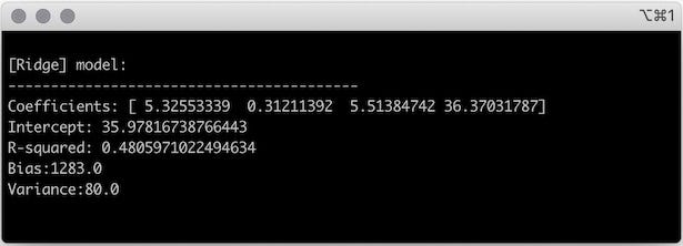
  Ridge regression was very effective at shrinking the value of the coefficients and, as a consequence, the variance of the model was significantly reduced.

  However, the complexity and interpretability of the model remained the same. You still have four features that impact the duration of your dog’s daily nap.

  Let’s turn to Lasso and see how it performs.

  Lasso

  Lasso is short for Least Absolute Shrinkage and Selection Operator [2], and it minimizes the sum of the absolute values of the coefficients.

  

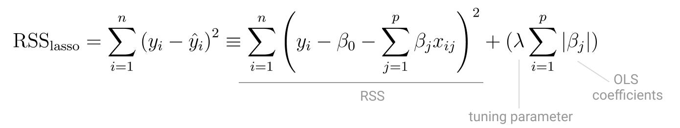
  It’s very similar to Ridge regression but, instead of the L2 norm, it uses the L1 norm as part of the shrinkage penalty. That’s why Lasso is also referred to as L1 regularization.

  What’s powerful about Lasso is that it will actually shrink some of the coefficients to zero, thus reducing both variance and model complexity.

  Lasso uses a technique called soft-thresholding[1]. It shrinks each coefficient by a constant amount such that, when the coefficient value is lower than the shrinkage constant it’s reduced to zero.

  Again, with an arbitrary lambda of 0.5, you can fit lasso to the data.

  In this case, you can see the feature squirrels was dropped from the model, because its coefficient is zero.

  

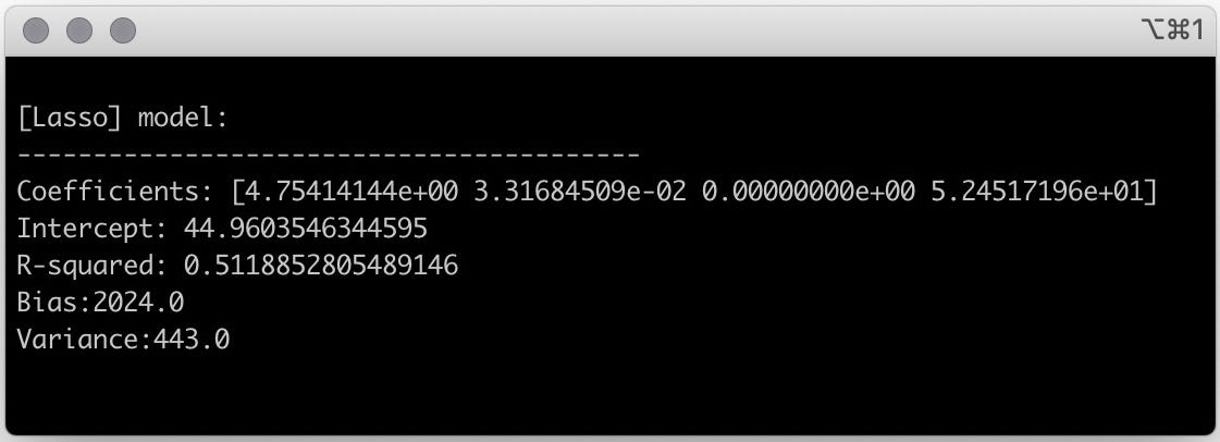
  With Lasso, your dog’s nap duration can be described as a model with three features:

  

  Here the advantage over Ridge regression is that you ended up with a model that is more interpretable, because it has fewer features.

  Going from four to three features is not a big deal in terms of interpretability, but you can see how this could extremely useful in datasets that have hundreds of features!

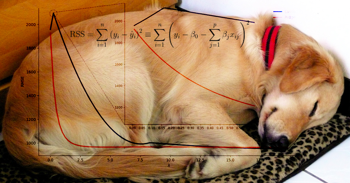
  Finding your optimal lambda

  So far the lambda you used to see Ridge Regression and Lasso in action was completely arbitrary. But there’s a way you can fine-tune the value of lambda to guarantee that you can reduce the overall model variance.

  If you plot the root mean squared error against a continuous set of lambda values, you can use the elbow technique to find the optimal value.